Digital vs Analog Simulation

While a purely digital simulation (Model-in-the-Loop) is great for testing logic, an analog simulation (Hardware-in-the-Loop) tests the electrical reality of your system. In a digital simulation, you use values like pressure directly from your atmosphere model. In reality, that pressure goes through a sensor which outputs voltage/current. Your electronics have to read that analog signal and convert it to digital before feeding it to your controller.

A real controller output has to drive a load. Analog simulation ensures the controller's transistors don't overheat or drop voltage when trying to move a high-pressure valve.

Your internal  Analog-to-Digital Converter (ADC) might add extra error. For example, your atmosphere model says 101.325kPa, but your ADC might convert it to 101.328 kPa due to its internal tolerance. Analog simulation reveals whether your control algorithm is robust enough to handle that 0.003 kPa error without oscillating. It also verifies that your controller’s ADC is actually calibrated correctly. The signal chain:

You cannot "short a wire to ground" in a purely digital simulation and see the smoke. With hardware like NI PXI Fault Insertion Units, you can physically short an analog input to a 24V rail. This allows you to verify that your hardware's protection diodes work and that your software enters a "Safe State" immediately.

Simulation variable names

In simulation, you have to be precise when talking about a parameter. For example, it is never enough to say "height". You should always say "height with respect to mean sea level, with units in feet". The reason is that height can also be measured from WGS84 ellipsoid or ground (AGL). Every couple of months, I see engineers waste days, sometimes weeks, due to such misunderstandings.

Here is a list that I frequently encounter, with bad and good variable naming:

• height: h - hMSL_ft (height measured from MSL, units in feet)
• time: t - timeFreeFlight_s (time started at free flight start, units in seconds)
• time: currentTime - currentTime_UnixEpoch_s (time started at Unix epoch, units in seconds)
• date: currentDate - currentDate_UTC (date in UTC)
• velocity: v - v_bc_Fn_mps (velocity of body fixed frame Fb wrt ground fixed frame Fc, with components expressed in NED frame, units in m/s)
• speed: v - speed_Mach
• acceleration: a - a_bi_noG_Fb_mps2 (acceleration of Fb wrt inertial frame Fi, without gravity components, expressed in Fb, units in m/s^2)
• Euler angles: euler - euler_Fn2FbRFB321_rpy_rad (321 yaw pitch roll sequence rotated frame based Euler angles that convert a vector in Fn to a vector in Fb, array index order is roll pitch yaw, units in radians)
• Azimuth: az - azimuthTrueNorth_deg (azimuth angle measured from True North, units in degrees)

Music: Peyk - Don Kafa

Finding root cause of latencies

A common issue in real-time hardware-in-the-loop simulations is latency in components that run on separate computers. These latencies can significantly degrade system performance. To differentiate between delays in component operations and network latency, you can send timestamps along with the data, log the time at reception, and record both timestamps:

Since components A and B have different clocks, you cannot directly compare the send and receive times. However, you can calculate the differences separately. If diff(timeSend) == diff(timeReceive), the latencies are likely not due to network congestion or a faulty switch/NIC but rather to delays in the operation of component A. It is highly unlikely for time differences to be the same if there is a problem with the network, it could only happen if the network was always adding a constant delay for each packet transmission.

Of course, you should perform the file saving in a separate thread to prevent blocking other operations. To minimize disk access, write to the log file periodically, for example, by flushing the log buffer to the file once per second.

When do you need HIL tests?

The steps to create an autonomous aircraft, from design to product, are as follows:

1. Concept of Operation
2. Requirements
3. Design
4. Ground tests
1. Test components
2. Test system
5. Flight tests
6. Deployment
7. Maintenance/Updates

As you progress through these steps, the cost of fixing problems increases exponentially.

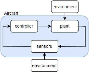
Consider a typical closed-loop diagram:

The "plant" consists of the airframe, actuators, and engine. The environment includes the atmosphere, aerodynamics, gravity, and electromagnetic interference.

During design phase, you start without any hardware and simulate everything with software-in-the-loop (SIL) simulations. The advantage of SIL is that it allows you to run millions of automated tests in a short time and with low cost to verify that you don't have any logic errors in your software. 

As hardware becomes available, you proceed to ground tests, transitioning more and more of your software from standard PCs to custom hardware. This slower and more costly step is called hardware-in-the-loop (HIL/HWIL) tests. HIL tests are necessary because:

1. Your system might work in SIL but since certain bugs only manifest themselves on a particular OS - compiler - hardware configuration, you cannot be sure with just SIL tests that your software is bug-free. Note: Instead of bug-free, the term 'tolerable' might be more appropriate because, for complex software, it is statistically improbable to achieve an entirely bug-free state.
2. Resource constraints (memory, processing power, network speed, etc.) of real hardware might differ from those in SIL which might cause a working system in SIL to fail in HIL due to missed timings etc.
3. Electromagnetic conditions (interference, noise, etc.) might differ from those in SIL. Components that work individually in isolation might cause problems when integrated together.
4. Although you can't test as extensively as with SIL, you can still conduct far more tests than with flight tests.

Music: Daydream In Blue

Avoiding catastrophic cancellation

Catastrophic cancellation occurs when subtracting two nearly equal numbers, leading to a significant loss of precision due to limited precision of floating-point numbers in a computer. Below are some examples and their better versions (reference):

log(a)−log(b) = log(a/b)

Computing cos(x)−1 for small values of x --> cos(x) ≈ 1−(x^2)/2 

Vertical Landing Rocket Competition

This year's Teknofest has a Vertical Landing Rocket Competition. We can divide the control problem into two:

1. Stabilize orientation so that the thruster points in downward direction.
2. Control vertical speed to achieve a soft landing.

Orientation can be stabilized via passive fins or active side jets. Since there isn't much time for manufacturing and testing, using fins seems to be the easiest choice.

Assuming that the fins achieve close to zero yaw and pitch, speed can be controlled by changing the thrust via valve control using PID.  I wrote a Matlab script that can be used as a starting point:

I also wrote a simple open loop code that has no control, you can find it here.

Applying derivative and integral on noisy data

Let's say you have a motion with sinusoidal acceleration, i.e. xddot(t) = sin(t). The analytic solution for speed and position will be xdot(t) = -cos(t)+1 (assuming zero initial speed) and x(t) = -sin(t) + t.  Let's say you don't know the analytical expressions of position, speed and acceleration and only have their values at a fixed sample rate. If you want to increase the samples, you can use Matlab's spline function.

If you have position as input and calculate speed and acceleration, if there is any noise in the signal, it will be amplified. If you have acceleration as input and calculate speed and position via integration, noise will be attenuated. Another advantage of using integration instead of derivation is that we can use linear interpolation since when integrating, we don't need smooth second derivatives. This both decreases computational load and lag due to two points in linear interpolation compared to four points in spline. See below Matlab code for an example:

HWIL development workflow

A typical HIL/HWIL development workflow starts with Simulink models and ends with code deployed on hardware with software that is expected to run in real time:

If there are differences between Simulink and Visual Studio runs, most of the time it is due to you forgetting to equalize all inputs. If you are sure about inputs being the same, the remaining sources of difference are details of floating point representations and sometime a block in Simulink generating wrong code. For example Aerospace blockset ECEF2LLA block code results in latitude lagging one time step behind, which does not occur during a Simulink run.

If there are differences between software running on hardware and Visual Studio results, it might be an indication of insufficient stack size allocation or tasks not meeting their deadlines. If you are lucky and have an advanced real time OS like VxWorks, it might throw a segmentation violation if there is too little stack available. If you don't want to count on luck, you have to test thoroughly, preferably using automated tests.